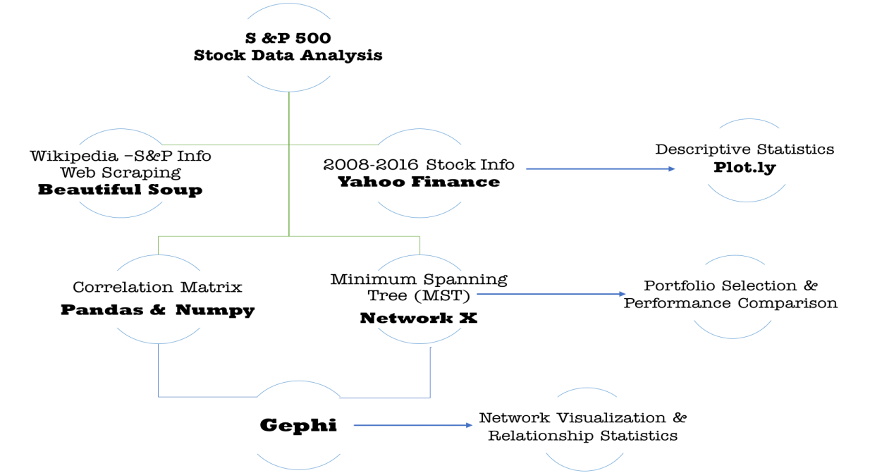
The Figure above displays a summary of our methodology. All Jupyter notebooks are available in the links provided in this page. Graphics within the notebooks are discussed in the Results section.

Data Summary

We started by web-scraping the S&P wikipedia page to get the name of the companies and the standard industrial calsssification code. The later helped us to classify the stocks into different sectors which will be ised in the visualization part. We then used the Yahoo Finance module to download the Closed Stock Price and Volume for ~250 days/year for 2008-2016. Dowloading the data takes about ~30 mins/per year, resulting in 4.5 hours period to download the data for 2008-2016. We created the Closed Price correlation matrix, and used this as a filtering method to determine relationship between the stocks.

#Piece of code to showcase written method used to download the daily closed price for all years

# Function to retrieve the daily close price for a specific stock from Yahoo Finance
def get_stockprice(ticker, start_date, end_date):
    """
    Return the daily adjusted close price of one stock in a certain period.
    Args:
    ticker(string): stock symbol of a company.
    start_date, end_date(string): time interval bounds in the format of 'yyyy-mm-dd'.
    """
    stock = Share(ticker)
    df = pd.DataFrame(stock.get_historical(start_date, end_date))
    df.index = df['Date']
    df.rename(columns = {'Adj_Close':ticker}, inplace = True)
    df[ticker] = pd.to_numeric(df[ticker])
    return df[ticker]

The jupyter notebook for the Data_Download is available here . In this other jupyter notebook you can find some interactive plots made in plot.ly to compare trends of stocksGraphics.ipynb

Network Construction

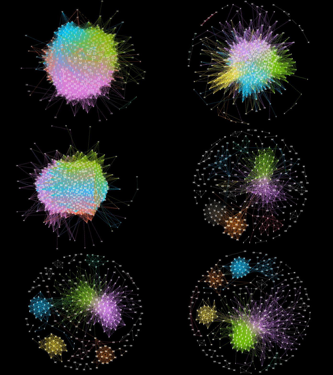
We decided to model the stock market as a network, where companies/stocks are respresented as a node. We proceeded to use the correlation matrix as a filtering method to define the interaction and create the edges between pairs of companies. Edges were created when the |correlation| between a \(stocks(i,j) > t\) where t is a pre-specified threshold. Although, there are modules that enable the creation of networks in python such as networkx and igraph, we decided to use Gephi available here to plot the visualizations due to its nice visualization features and automatic production of network related statistics. Summary graphics done from the relatedness statistics were done using matplotlib and plot.ly can be found here Statistical Analysis.ipnyb

Minimum Spanning Tree

Minimum Spanning Trees (MST) are undirected graphs with weights on the edges. We used the correlation matrix in a different form by transforming into distances through the use of the equation: \(distance[i, j] = sqrt(2.0 * ( 1 – correlation[i, j] )\) . MST was used to select a portfolio (set of stocks) based on centrality and distance measures. Peripheral portfolio was done by selecting stocks with greater distance in between them, and central portfolio by selecting stocks that have more the edges associated with its node. Peripheral stocks do not necessarily posses relationship between each other. We also computed relationship statistics and provided performance comparison of our selected portfolio againts the market for 2016.

More information about how we computed the MST here: https://verali0816.github.io/Stock-Correlation/MST

#Method written in python to develop the MST

def minimum_spanning_tree(X, copy_X=True):
    """X are edge weights of fully connected graph"""
    if copy_X:
        X = X.copy()
 
    if X.shape[0] != X.shape[1]:
        raise ValueError("X needs to be square matrix of edge weights")
    n_vertices = X.shape[0]
    spanning_edges = []
     
    # initialize with node 0:                                                                                         
    visited_vertices = [0]                                                                                            
    num_visited = 1
    # exclude self connections:
    diag_indices = np.arange(n_vertices)
    X[diag_indices, diag_indices] = np.inf
     
    while num_visited != n_vertices:
        new_edge = np.argmin(X[visited_vertices], axis=None)
        # 2d encoding of new_edge from flat, get correct indices                                                      
        new_edge = divmod(new_edge, n_vertices)
        new_edge = [visited_vertices[new_edge[0]], new_edge[1]]                                                       
        # add edge to tree
        spanning_edges.append(new_edge)
        visited_vertices.append(new_edge[1])
        # remove all edges inside current tree
        X[visited_vertices, new_edge[1]] = np.inf
        X[new_edge[1], visited_vertices] = np.inf                                                                     
        num_visited += 1
    return np.vstack(spanning_edges)

Notebook for the creation of MST,selection of portfolio and performance graphics can be found here